Logistic Regression: A Classifier With a Sense of Regression

Explaining logistic regression as a classifier derived from regression concept.

Photo by d kah on Unsplash

Logistic Regression

You may have heard about the linear regression, given the features on datasets, you could predict the output labels using a linear regression derived from this linear equation

Equation 1. Linear Equation. Image by the Author

where:

Yi=the predicted label for the ith sample

Xij=the jth features for the ith-label

W0=the regression intercept or weight

Wj=the jth feature regression weight

The predicted labels are continuous numbers.

Logistic Regression is a supervised classifier of machine learning. In a classification problem, the prediction label can take only discrete values for a given set of features. Although commonly known as a classifier, Logistic Regression is a regression model

Just like Linear regression assumes that the data follows a linear equation in Equation 1. In Logistic Regression, the data follow the sigmoid function.

Equation 2. Sigmoid Function. Image by the Author

Sigmoid function graph. Image by vcal.com

Some important properties of sigmoid function f(z) :

1. f(z) is close to 0 when z → -∞
2. f(z) is close to 1 when z → +∞
3. f(z) equal to 1/2 when z=0 (the threshold)

Thus, the sigmoid function has 0 for the lower bound and 1 for the upper bound. Based on these properties, we compute the probability of a predicted label between an interval of 0 and 1. So if a computed probability of a label is greater than a threshold number, then it belonged to some class or category, otherwise, if it's less than the threshold number, it belongs to another class.

Hypothesis Function

In the case of logistic regression, we want our output as a probability bound to intervals of 0 and 1, and the input is in range(−∞,∞).

To transform the scale of the input into a probability between 0 and 1, we apply a mapping function. For the logistic regression model, this mapping function is the logit function. The logit function maps probabilities from the range (0,1) to the entire real number range (−∞,∞). It is written as

Equation 3. Logit Function. Image by The Author

Where y (hat) =the probability of the output

Supposedly, we have a set of input ranges (−∞,∞) in the form of linear equations:

Equation 4. Image by The Author

With the right-hand side equation being the matrix form. The logit function η can be written as:

Equation 5. The logit function. Image by the Author

Where:

W = weight matrix of j features

X = features matrix of i labels

Y = predicted labels matrix of i samples

Now we have a function to maps the probability of the output to the entire input. Interestingly, if we take the inverse of the logit function

Equation 6. Inverse Logit function. Image by the Author

Thus,

Equation 7. Hypothesis function of Logistic Regression. Image by the Author

We get the Sigmoid Function as the hypothesis function of Logistic Regression.

Cost Function

We already learnt about cost function J(w) for linear regression in the form of

Equation 8. Image by the Author

By applying the Gradient Descent we could get the optimum values of the weights w.

Convex Function

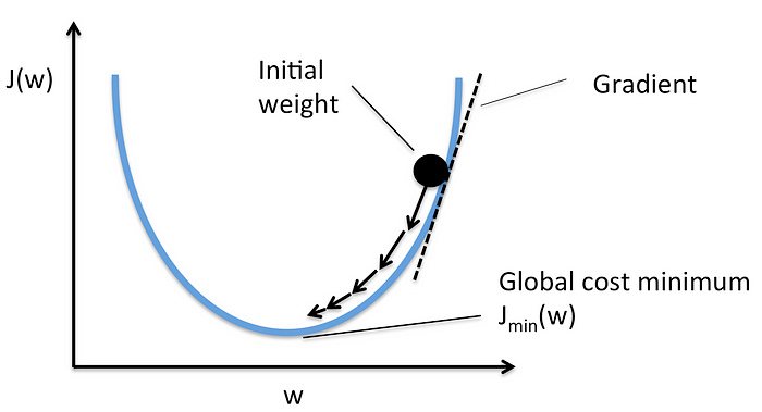
For Logistic Regression, if we use the cost function of linear equation, we would end up in non-convex function with many local minimum. It would be difficult to minimize the cost function and reach the optimum weight.

Convex and Non Convex Function. Image by Jennifer Rexford

To define the cost function for Logistic Regression, let's assume that our hypothesis equation in Logistic Regression is the conditional probability of finding the output label between 0 and 1. Given the feature x, weight w, and known label y of i-th observation, we define probability P as:

Equation 9. Probability of predicted label for known labels 1 and 0. Image by The Author

In general, the Probability P can be expressed using binomial distribution with n=1:

Equation 10. Probability of predicted labels . Image by The Author

Practically, we already got features x and known label y from the datasets, in order to maximize the probability of P, we need to choose the optimum weight to maximize the Likelihood of the predicted label. Likelihood define as

Equation 11. Likelihood Function, image by the Author

for easier calculation, let's rewrite Likelihood Function in logarithmic form log(L(w)=(l(w)), commonly known as Log-Likelihood

Equation 12. Log-Likelihood Function. image By the Author

Now, you might be guessing if the Log-Likelihood function is the cost function for Logistic Regression? well, it could be it. But, our goals are to apply Gradient Descent to the cost function, the shape of the curve of the Log-Likelihood is a bell-like shape, it’s increasing toward maximum value. on the contrary, the Gradient Descent iteratively finds the minimum of the curve, like a quadratic function. So we have to invert the Log-Likelihood. The inverted Log-Likelihood is also called Cross-Entropy. Therefore, our cost function is written as a function of Cross-Entropy.

Equation 13. Cost function of Logistic Regression. image by The Author

Gradient Descent

We are going to run Gradient Descent in a similar way like we already did for linear regression. It involves the gradient of the cost function and learning rate. The step to update the weights given by

Equation 14. weight iteration. image by the Author

The main different is the gradient of the cost functions, because we are using the Cross-Entropy as the cost function. We will not get into the detail of how to derive the gradient of the cost functions. Here are the gradient of the cost function.

Equation 15. Gradient of the cost function. image by the Author

Using the matrix form:

Equation 16. matrix form of the gradient of the cost function. image by the Author

Then, the steps to update weight:

Equation 17. weight matrix iteration. image by the Author

Where α is the learning rate.

Next, we will build the Logistic Regression using Python.

Implementation

Recall the model we wrote for the Multiple Linear Regression.

We’re going to modify the code, so it will work for Logistic Regression cases. First, change the class name to LogisticRegression.

We will be using the Sigmoid function as the hypothesis, let's define the method:

Modify the iteration in the fit method by following these steps:

1. For iteration 1 until n (the class iters property)
2. Compute the predicted labels matrix using Equation 7
3. Compute the gradient of the cost function using Equation 16
4. Update the weight matrix using Equation 17

Finally, modify the predict method by adding threshold argument. This will be used to get the category of the predicted labels. The steps are:

1. Calculate the predicted labels using equation 7
2. If the predicted labels > threshold return 1, otherwise is 0

This is the complete code of the model.

Let's test the model. We are going to use the breast cancer Wisconsin dataset. This dataset contains measurements of breast tissue. The goal is to determine whether a tumor is benign (harmless ) or malignant (that is dangerous, this is cancer). The Benign class is encoded as 1, otherwise the malignant class is encoded as 0. As the data comes with Scikit-learn, we can load it directly from the library. After the dataset been loaded, split the dataset into train and test datasets.

Now, let’s predict the labels:

To find out the accuracy of the predictions, use the built-in accuracy_scorefrom Scikit-learn:

The output is:

0.9298245614035088

The accuracy score produced the number around 0.93. This is quite good.

Conclusion

In this article, we have learned:

1. The Logistic Regression as a machine learning classifier algorithm, derived from the concept of Regression.
2. Deriving the cost function for Logistic Regression by utilizing the Cross-Entropy function
3. Implementing the Gradient Descent on Logistic Regression.

Please, share this post and give it a clap if you like it.

More content at PlainEnglish.io. Sign up for our free weekly newsletter. Follow us on Twitter and LinkedIn. Join our community Discord.